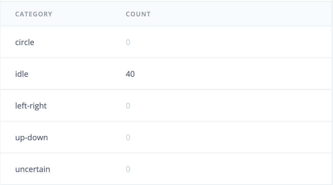
- idle: Only miniscule fluctuations in the sensor data, otherwise data readings constant
- circle: Device is moved in a circle motion. All accelerometers oscillate
- left-right: Acceleration on y-axis and x-axis, while z-axis (height acceleration) is calm. Moving object in different orientation in a plane. However, we have gyro acceleration around the z-axis
- up-down: Depending on how cleanly the up and down movement is performed we see oscillations in the magnetometers or not. The accelerometers are slighlty activated
All modes would be expected to only show in the acceleration data, but the device seems to have been rotated during data collection and some movement leaks into the other axis
Question 2. Your data doesn’t only include movements but also idle data. Why might it bebeneficial to include idle data?
To differentiate between moving and not moving. If there is no label/data for idle our model always outputs a movement, even though the confidence would be very low.
Question 3. Which settings did you choose in the Time series data input block? Explain what these settings do and why you think that your choices are a good choice. It might be a good idea to look at the patterns present in your data.
The window size is the length of one sample. It should be long enough to detect the movement so longer than one wavelength for a typical movement. We chose a window size of 2000ms since the typical movment seems to have a wavelength of about 1000ms so 2000ms should be enough to capture detect it.
The stride is the step size in ms at which data from the window is processed. If the step size is larger than the window we ignore data.
The frequency of the data is up or down sampled. since we have quite a slow movement, we are not expecting high frequencies so therefore we can downsample the data a bit to 50 Hz to have less input features and therefore less computational load.
Question 4. What do the different preprocessing blocks do? Briefly explain them. Why should we use preprocessing blocks instead of feeding the data directly into the neural network like using the raw preprocessing block?
- Spectral Features: Moves data from time domain into frequency domain
- Flatten: "The Flatten block first rescales axes of the signal if value is different than 1. Then statistical analysis is performed on each window, computing between 1 and 8 features for each axis, depending on the number of selected methods."
- Raw Data: Does not perform any processing and feeds the raw data directly to the model
In general, preprocessing is much less computationally intense compared to a (D)NN. If there a patterns or features in the model we know beforehand preprocessing can help to reduce the size of the model drastically while maintaining good performance.
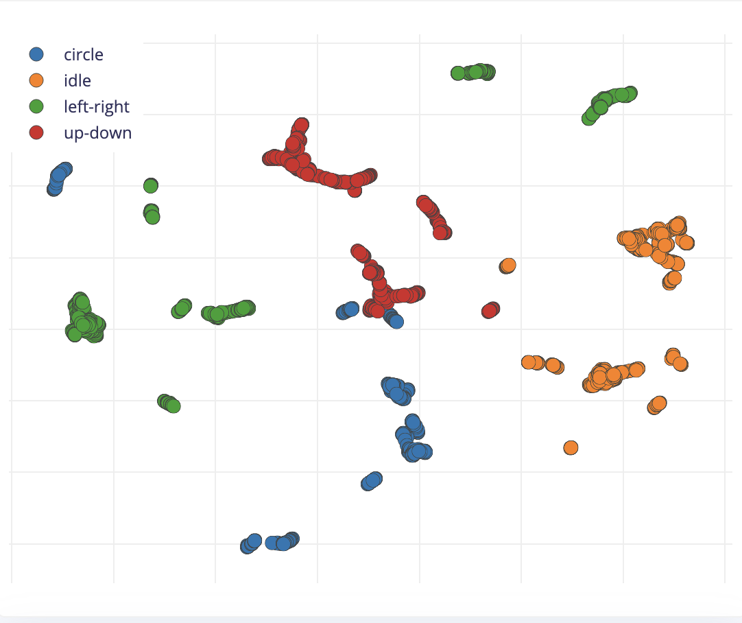
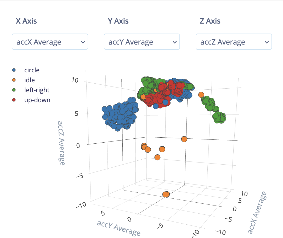
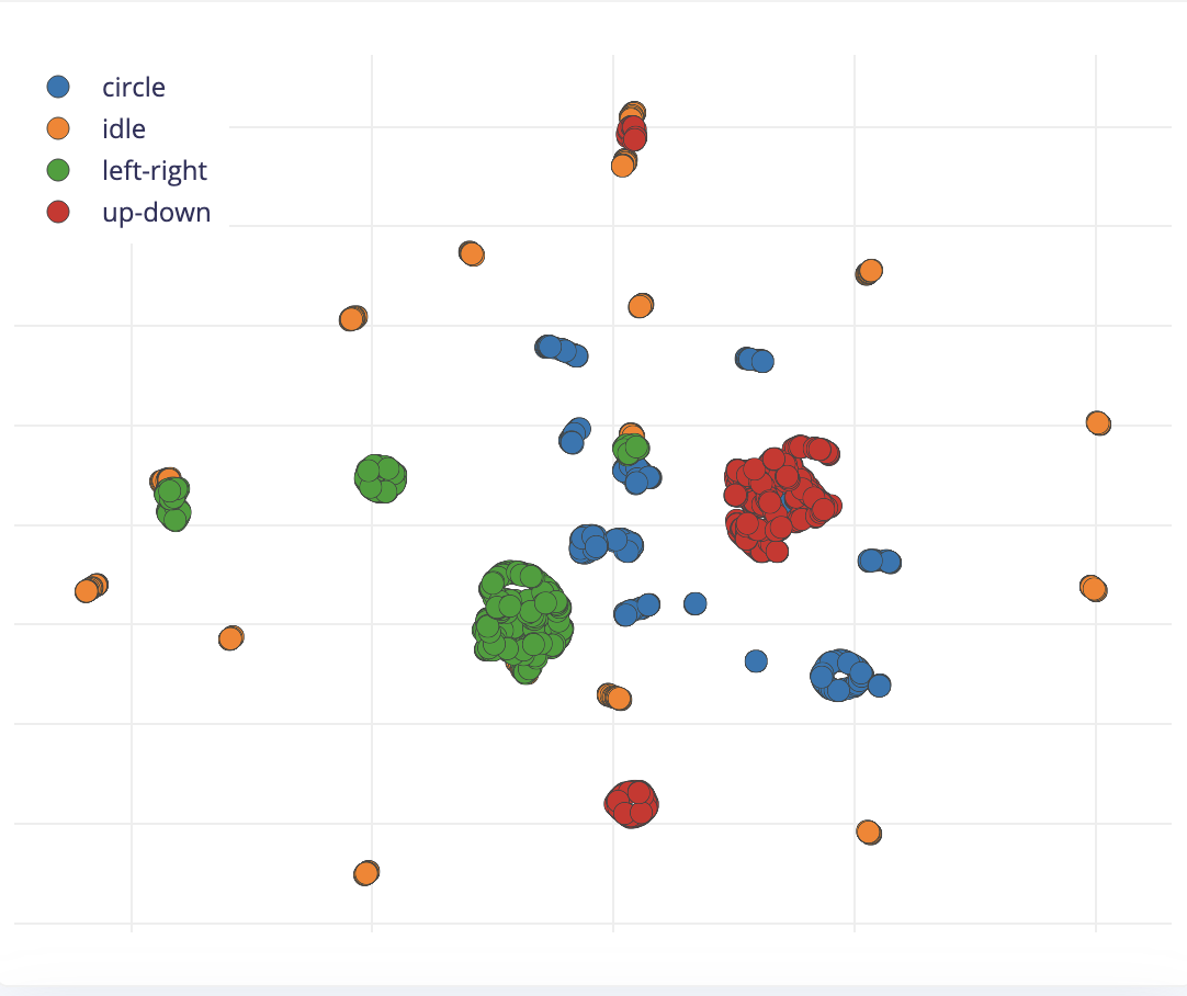
Question 5. Which preprocessing block creates the best features separating the classes? Add screenshots from the feature explorer. What kind of features did the blocks extract?
| Aspect | 1D Convolution | 2D Convolution |
|---|---|---|
| Input type | Sequential data | Image or spatial data |
| Kernel shape | 1D (e.g., 3) | 2D (e.g., 3×3) |
| Sliding direction | Along one axis (e.g., time) | Along two axes (height and width) |
| Feature extraction | Temporal or sequential features | Spatial features |
Question 7. Briefly explain your models. Is there anything special? Include the code for your models in your submission.
- Cycles: 30
- Learned Optimizer: [ ]
- Learning Rate 0.0005
Prepocessing: Spectral
model = Sequential()
model.add(Dense(20, activation='relu',
    activity_regularizer=tf.keras.regularizers.l1(0.00001)))
model.add(Dense(10, activation='relu',
    activity_regularizer=tf.keras.regularizers.l1(0.00001)))
model.add(Dense(classes, name='y_pred', activation='softmax'))
Prepocessing: Spectral
model = Sequential()
model.add(Dense(64, activation='relu',
    activity_regularizer=tf.keras.regularizers.l1(0.00001)))
model.add(Dense(32, activation='relu',
    activity_regularizer=tf.keras.regularizers.l1(0.00001)))
model.add(Dense(classes, name='y_pred', activation='softmax'))
Prepocessing: Spectral
model = Sequential()
model.add(Dense(128, activation='relu',
    activity_regularizer=tf.keras.regularizers.l1(0.00001)))
model.add(Dense(64, activation='relu',
    activity_regularizer=tf.keras.regularizers.l1(0.00001)))
model.add(Dense(32, activation='relu',
    activity_regularizer=tf.keras.regularizers.l1(0.00001)))
model.add(Dense(classes, name='y_pred', activation='softmax'))
Preprocessing: Raw Data
model = Sequential([
    Conv1D(16, kernel_size=5, activation='relu', input_shape=(627,1)),
    BatchNormalization(),
    MaxPooling1D(pool_size=2),

    Conv1D(32, kernel_size=5, activation='relu'),
    BatchNormalization(),
    MaxPooling1D(pool_size=2),

    Flatten(),

    Dense(32, activation='relu', kernel_regularizer=tf.keras.regularizers.l2(1e-4)),
    Dropout(0.3),

    Dense(classes, activation='softmax', name='y_pred')
])
Preprocessing: Raw Data
model = Sequential([
    Conv1D(8, kernel_size=5, activation='relu', input_shape=(627,1)),
    BatchNormalization(),
    MaxPooling1D(pool_size=2),

    Conv1D(16, kernel_size=5, activation='relu'),
    BatchNormalization(),
    MaxPooling1D(pool_size=2),

    Flatten(),

    Dense(16, activation='relu', kernel_regularizer=tf.keras.regularizers.l2(1e-4)),
    Dropout(0.3),

    Dense(classes, activation='softmax', name='y_pred')
])
Preprocessing: Raw Data
model = Sequential([
    Conv1D(8, kernel_size=5, activation='relu', input_shape=(627,1)),
    BatchNormalization(),
    MaxPooling1D(pool_size=2),

    Flatten(),

    Dense(16, activation='relu', kernel_regularizer=tf.keras.regularizers.l2(1e-4)),
    Dropout(0.3),

    Dense(classes, activation='softmax', name='y_pred')
])
Preprocessing: Raw Data
model = Sequential([
    Conv1D(8, kernel_size=5, activation='relu', input_shape=(627,1)),
    BatchNormalization(),
    MaxPooling1D(pool_size=2),

    Conv1D(16, kernel_size=5, activation='relu'),
    BatchNormalization(),
    MaxPooling1D(pool_size=2),

    Flatten(),

    Dense(classes, activation='softmax', name='y_pred')
])
Preprocessing: Raw Data
model = Sequential([
    Conv1D(4, kernel_size=5, activation='relu', input_shape=(627,1)),
    BatchNormalization(),
    MaxPooling1D(pool_size=2),

    Conv1D(8, kernel_size=5, activation='relu'),
    BatchNormalization(),
    MaxPooling1D(pool_size=2),

    Flatten(),

    Dense(classes, activation='softmax', name='y_pred')
])
Preprocessing: Raw Data
model = Sequential([
    Conv1D(16, kernel_size=5, activation='relu', input_shape=(627,1)),
    BatchNormalization(),
    MaxPooling1D(pool_size=2),

    Flatten(),

    Dense(classes, activation='softmax', name='y_pred')
])
Preprocessing: Raw Data
model = Sequential([
    Conv1D(8, kernel_size=5, activation='relu', input_shape=(627,1)),
    BatchNormalization(),
    MaxPooling1D(pool_size=2),

    Flatten(),

    Dense(classes, activation='softmax', name='y_pred')
])
Question 8. What is the training performance of the models? How much memory is your model expected to need? What execution time is estimated? You can add screenshots. Check also for the memory usage and execution time of your DSP blocks.
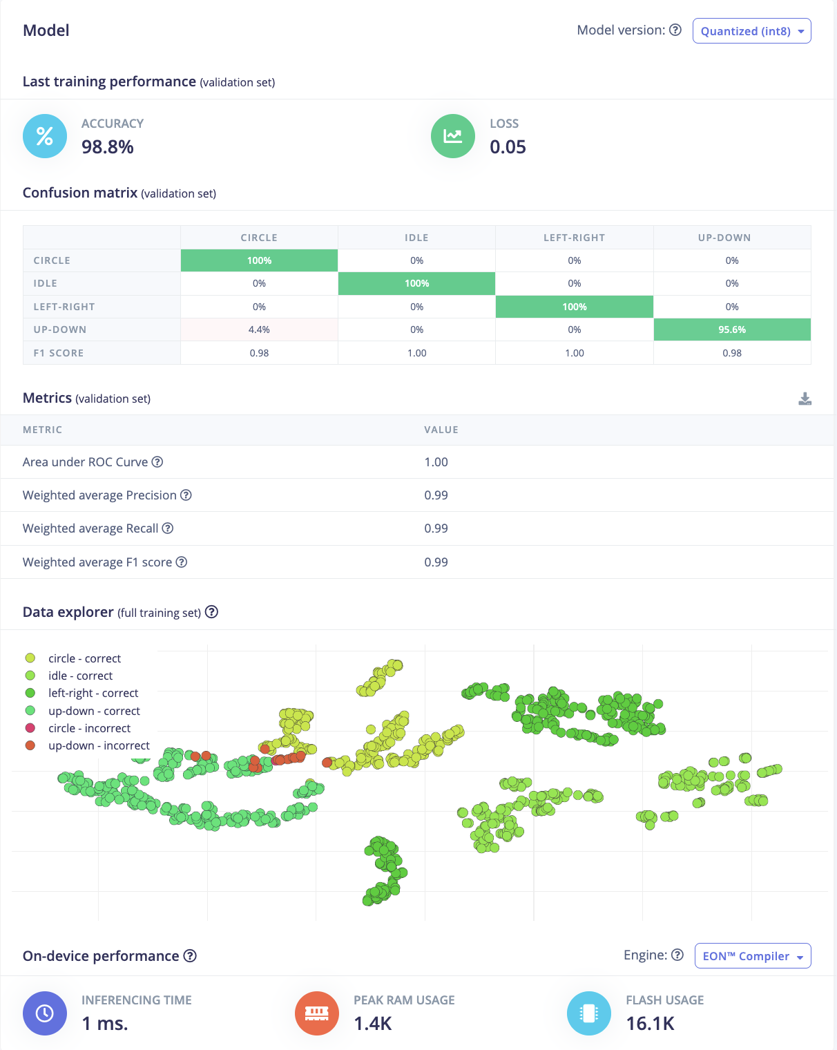
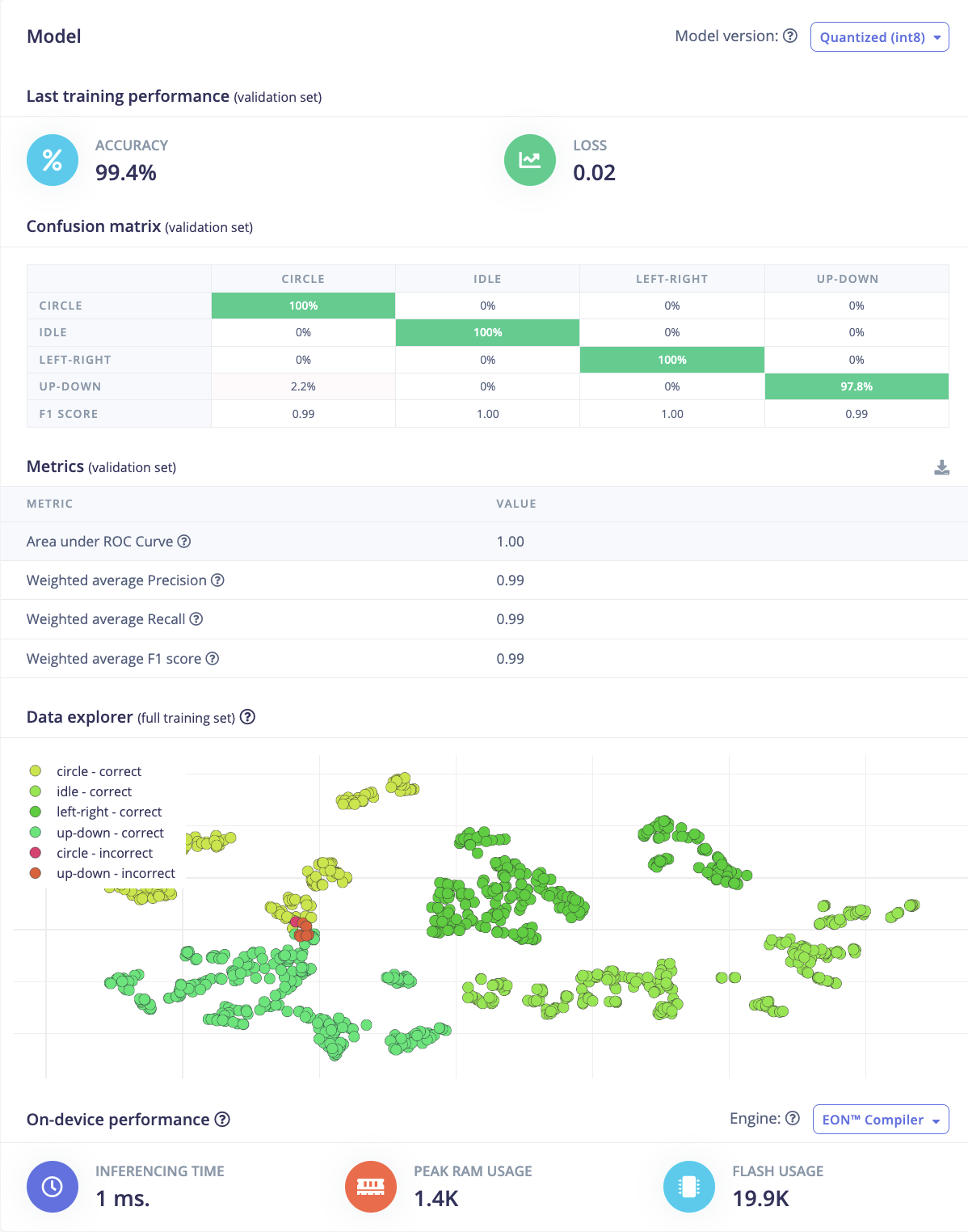
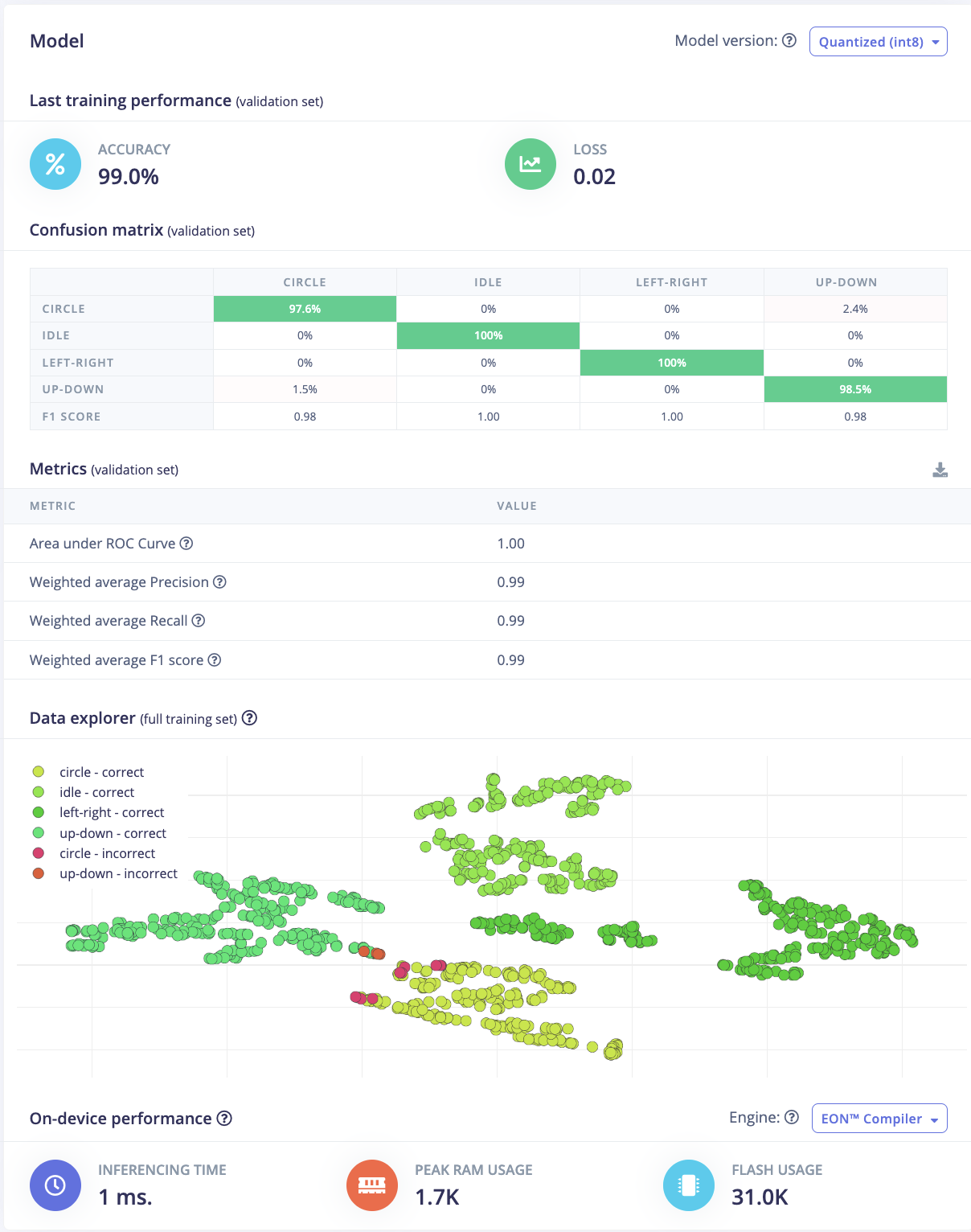
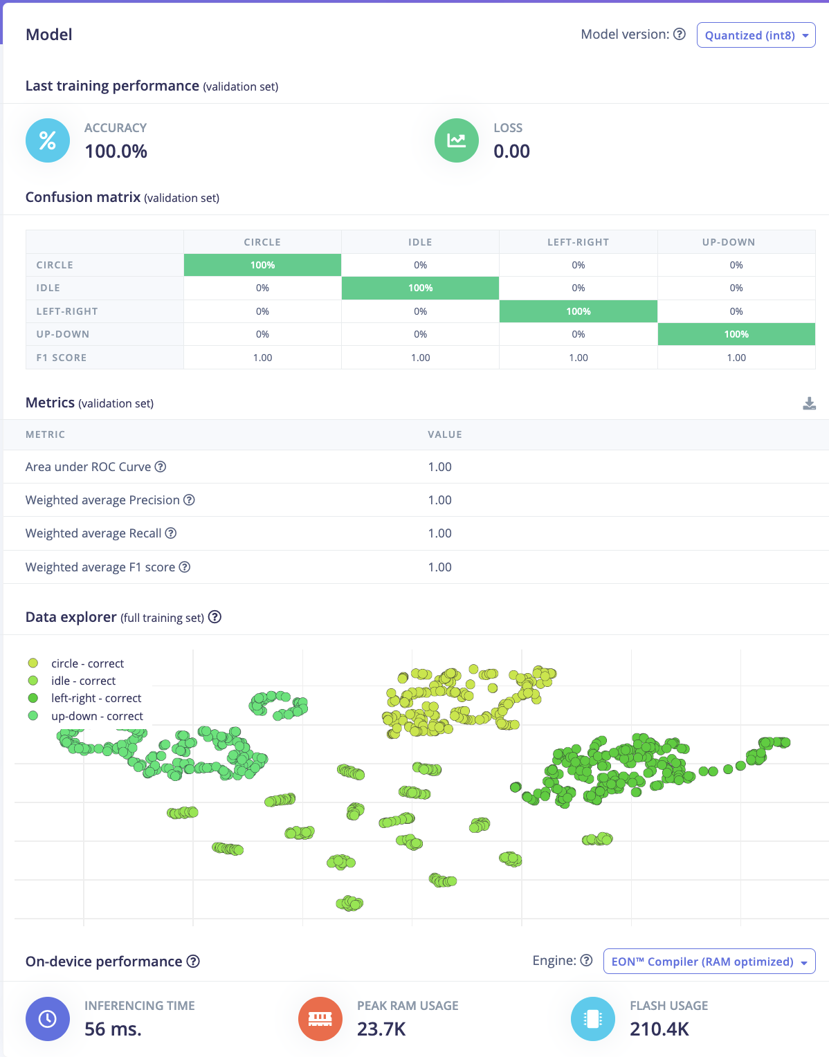
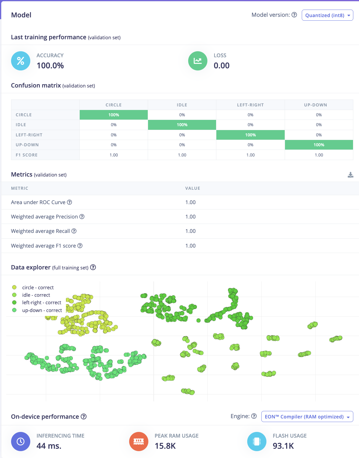
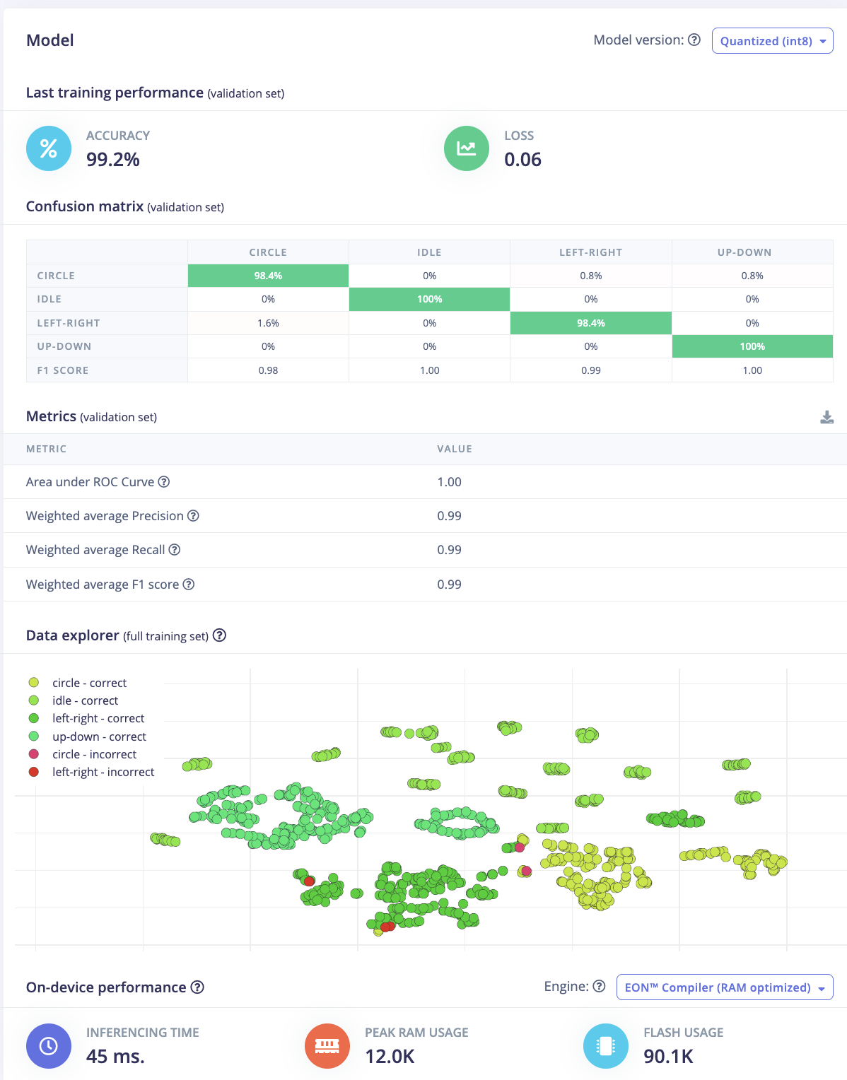
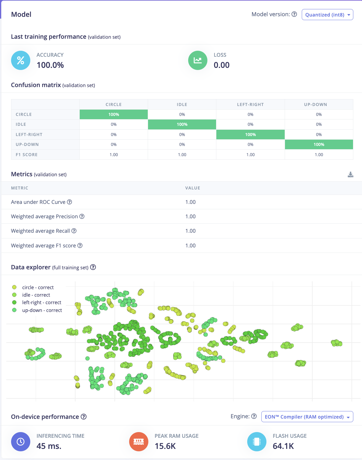
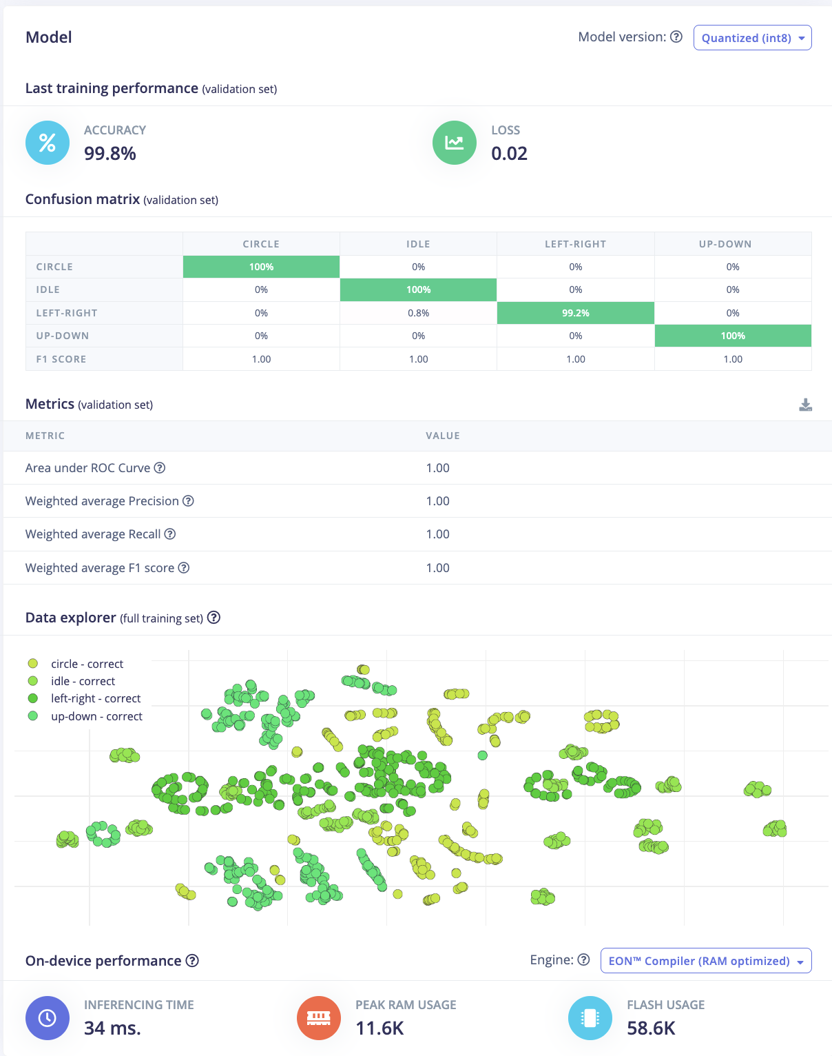
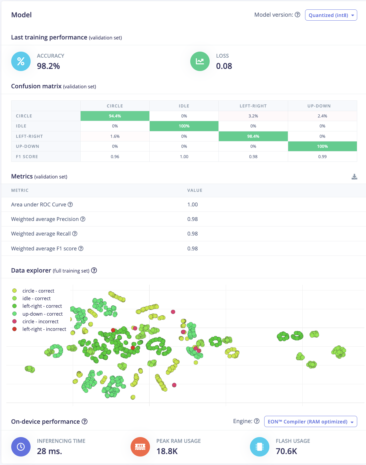
Despite really good training accuracy of 98%! -> Bad generalization
Question 9. How good do your models classify the test data? Do the models generalize well? Create plots (bar graphs) comparing your models. Also explain F1 Score and Uncertainty displayed in the confusion matrix.
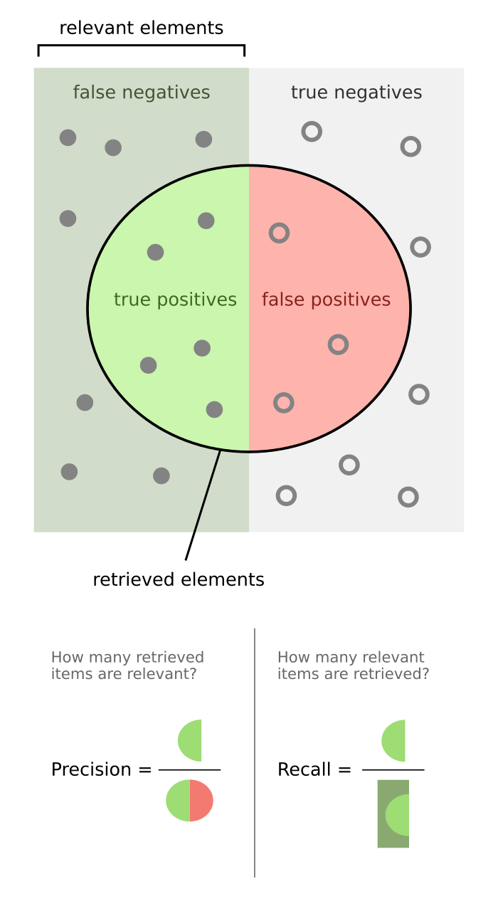

- F1-Score: "The F1 score is the harmonic mean of the precision and recall. It thus symmetrically represents both precision and recall in one metric."
- Uncertainty: Removed from confusion matrix
| Model | Preprocessing | Accuracy (%) | Inference Time (ms) | RAM usage (bytes) | Flash Usage (bytes) |
|---|---|---|---|---|---|
| Dense | spectral | 98.8 | 1 | 1.4K | 16.1K |
| Dense Wide | spectral | 99.4 | 1 | 1.4K | 19.9K |
| Dense Wide+Deep | spectral | 99.0 | 1 | 1.7K | 31K |
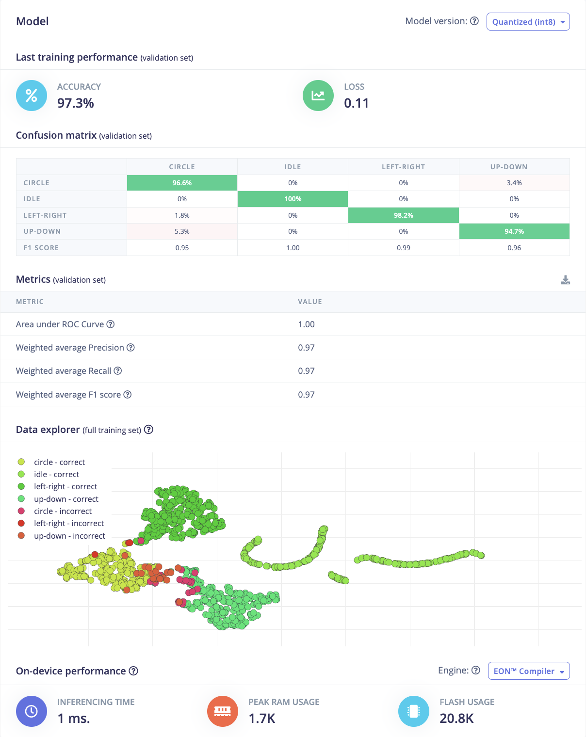
| Dense EON | spectral | 97.3 | 1 | 1.7K | 20.8K |
| CNN+Dense Large | raw | 100 | 56 | 23.7K | 210K |
| CNN+Dense Small | raw | 100 | 44 | 15.8K | 93.1K |
| CNN+Dense Tiny | raw | 99.2 | 45 | 12K | 90.1K |
| CNN | raw | 100 | 45 | 15.6K | 64.1K |
| CNN Small | raw | 99.8 | 34 | 11.6K | 58.6K |
| CNN Tiny | raw | 98.2 | 28 | 18.8K | 70.6K |
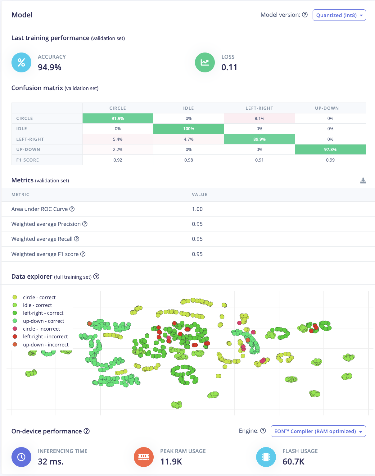
| CNN Micro | raw | 94.9 | 32 | 11.9K | 60.7K |
Question 10. Did the EON Tuner come up with a better model than you? If so, in which regard is it better? Is it still better when you limit it to using only accelerometer data? (To answer the latter question, first answer Question 11.)
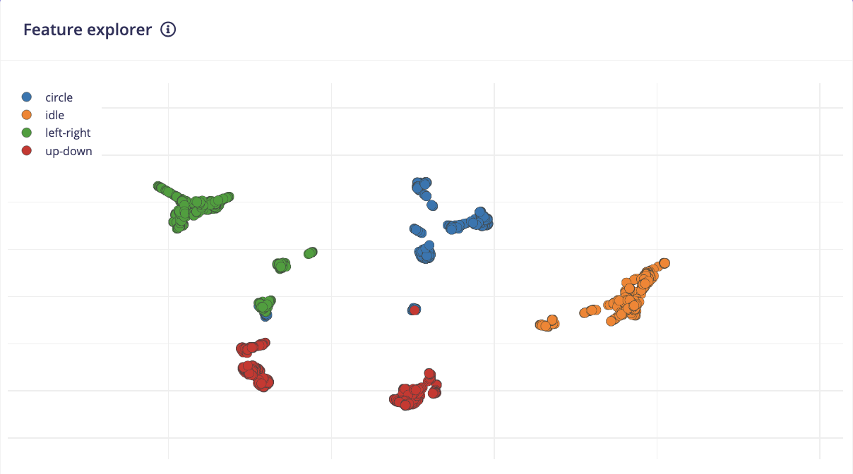
Nice separation of features
model = Sequential()
model.add(Dense(40, activation='relu',
    activity_regularizer=tf.keras.regularizers.l1(0.00001)))
model.add(Dense(20, activation='relu',
    activity_regularizer=tf.keras.regularizers.l1(0.00001)))
model.add(Dense(10, activation='relu',
    activity_regularizer=tf.keras.regularizers.l1(0.00001)))
model.add(Dropout(0.5))
model.add(Dense(classes, name='y_pred', activation='softmax'))

After removal of all features except accelerometer data it performs worse:
Question 11. If the EON tuner resulted in a better model, add this model as a new impulse and use it as well in the Model Testing section, and add its results to the plots you created in Question 9. Please note: Before doing so, save your current version with the versioning tool on the left.
Question 12. Explain the output of the classification results. Does your model work? Did it misclassify some timestamps? Is this a bad thing? Why (not)?
Question 13. Does the classification also work for your phone? If it doesn’t work, why not? Does the performance change when you change the orientation of your phone? In which orientation do you have to hold your phone for it to work best?
- Phone orientation: Flat
- Movement: Circle
- Classification: Up-Down
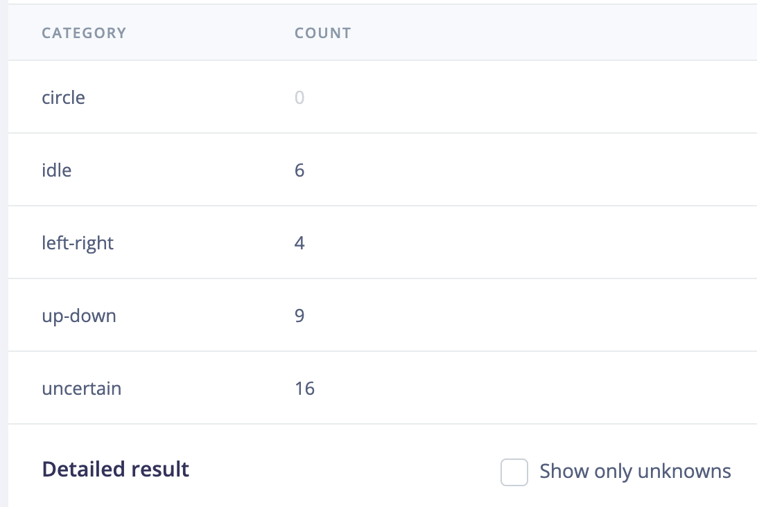
- Phone orientation: Upright
- Movement: Circle
- Classification: Left-Right
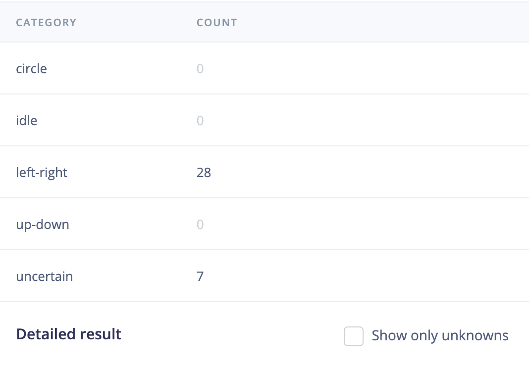
- Phone orientation: Flat
- Movement: Up-Down
- Classification: Idle
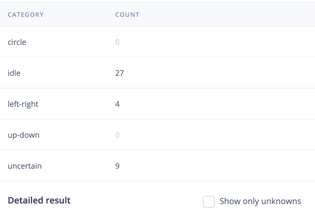
- Phone orientation: Upright
- Movement: Up-Down
- Classification: Left-Right
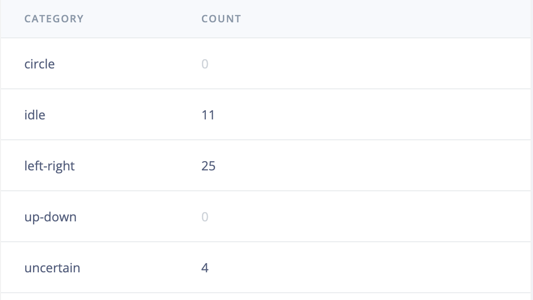
- Phone orientation: Flat
- Movement: Left-Right
- Classification: Left-Right
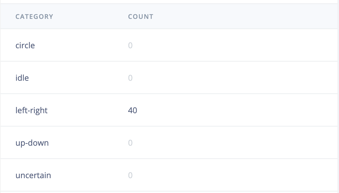
- Phone orientation: Flat, upside-down
- Movement: Up-Down
- Classification: Up-Down
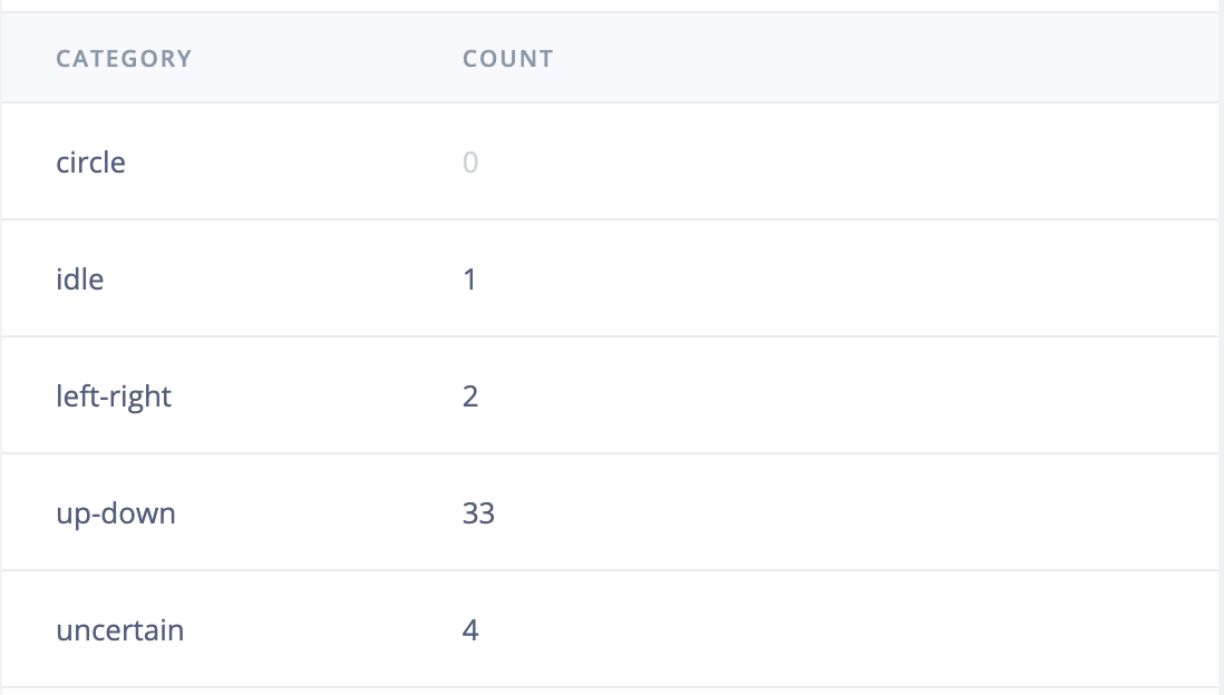
- Phone orientation: Flat, upside-down
- Movement: None
- Classification: Idle