- simulation_source_connectivity
MATLAB function that allows to generate pseudo-EEG signals imposing a three-nodes brain network used for the evaluation of:
- two different methods for the brain source localization, the Exact Low Resolution Tomography (eLORETA) and the Linearly Constrained Minimum Variance (LCMV) beamformer;
- the impact of the demixing approach on the connectivity estimates performed by Multivariate Granger Causality (MVGC), Time Reversed Granger Causality (TRGC) and Partial Directed Coherence (PDC).
The code allows to set different parameters such as the “alpha” related with the Signal to Noise Ratio (SNR), the type of moving dipole (Interactive or Non-interactive) and the position of the fixed dipole that can be:
- Far superficial: dipoles located far from each other’s and near the cortex;
- Far deep: dipoles located far from each other’s and deep in the brain;
- Close superficial: dipoles located close from each other’s and near the cortex;
- Close deep: dipoles located close from each other’s and deep in the brain.
The moving dipole change over 1004 positions within the brain.
Firstly, the function “generate_MVARdata” generates three time-series (variable “Y”) on the basis of the ground-truth connectivity pattern imposed in the variable “model” (3x3 matrix whose elements are “1” to indicate an existing connection between two nodes). The function “mkpinknoise” provides the generation of 500 biological noisy sources (variable “pn”).
Both, brain signals and noise, are projected and summed on the scalp considering a specific SNR. The forward model is solved according to the New York Head Model, whose parameters are contained in the structure “sa_v2”. It was obtained from the “sa” structure available on the ICBM-NY platform.
A simulated measurement noise is also added at sensor level according with the toolbox developed by Haufe and Ewald available at http://bbci.de/supplementary/EEGconnectivity/BBCB.html [1].
As mentioned before, the source reconstruction is performed employing two different approaches:
- eLORETA algorithm (function “mkfilt_eloreta2”), providing the reconstructed sources contained into the variable “H” [2];
- LCMV algorithm (function “mkfilt_lcmv”) [3].
The connectivity estimates are then performed on the reconstructed time series:
- MVGC is computed according to the Seth and Barnett Toolbox (function “GCCA_tsdata_to_pwcgc”) that is possible to download at http://www.sussex.ac.uk/sackler/mvgc/ [4].
- TRGC is performed by means of the function “tr_gc_test” (implemented by us)[5].
- PDC is performed according to the toolbox implemented by Baccalà et al. (functions “mvar” and “asymp_PDC”). It is free and available at http://www.lcs.poli.usp.br/~baccala/pdc/ [6].
The comparison between the obtained connectivity binary matrix and the imposed model allow to evaluate the False Positive Rate (FPR), the False Negative Rate (FNR) and the Area Under the ROC Curve (AUC) parameters.
Each simulated condition is iterated for the 1004 different positions of the moving dipole. A block diagram reporting the main steps of the simulation framework is reported in the following figure
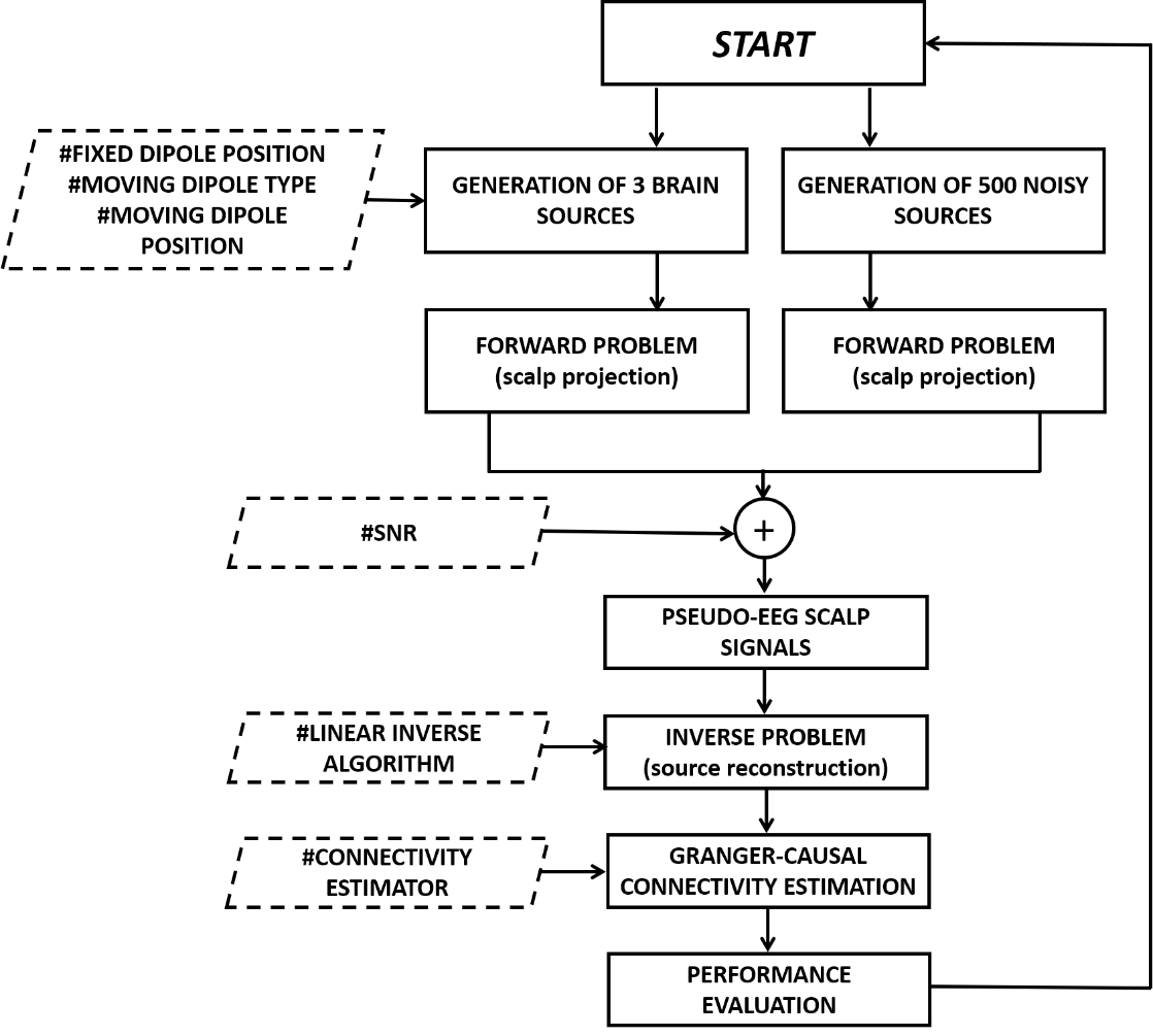
The obtained results and the set parameters are stored and saved into a structure called “Simulation”. The dipole locations into a structure called "Location".
- run_simulation_source_connectivity
MATLAB script that allows to run the main function “simulation_source_connectivity” after imposing the parameters:
- type of moving dipoles
- positions of the fixed dipoles
- SNR
- number of iterations
- brain_maps_FPR
MATLAB script for the visualization of the simulations results in terms of FPR on a 3-D head model. To run this code it is necessary to add ONLY the folder "plotting" of the FieldTrip toolbox to the set path (free download at http://www.fieldtriptoolbox.org/download)
- movie_rotating_FPR
MATLAB script able to create a movie in which the figure obtained from the previous script rotate along the main axes.
[1] S. Haufe e A. Ewald, «A Simulation Framework for Benchmarking EEG-Based Brain Connectivity Estimation Methodologies», Brain Topogr., pagg. 1–18, giu. 2016.
[2] R. D. Pascual-Marqui et al., «Assessing interactions in the brain with exact low-resolution electromagnetic tomography», Philos. Transact. A Math. Phys. Eng. Sci., vol. 369, n. 1952, pagg. 3768–3784, ott. 2011.
[3] B. D. Van Veen, W. van Drongelen, M. Yuchtman, e A. Suzuki, «Localization of brain electrical activity via linearly constrained minimum variance spatial filtering», IEEE Trans. Biomed. Eng., vol. 44, n. 9, pagg. 867–880, set. 1997.
[4] L. Barnett e A. K. Seth, «The MVGC multivariate Granger causality toolbox: a new approach to Granger-causal inference», J. Neurosci. Methods, vol. 223, pagg. 50–68, feb. 2014.
[5] S. Haufe, V. V. Nikulin, K.-R. Müller, e G. Nolte, «A critical assessment of connectivity measures for EEG data: A simulation study», NeuroImage, vol. 64, pagg. 120–133, gen. 2013.
[6] K. Sameshima, D. Y. Takahashi, e L. A. Baccalá, «On the statistical performance of Granger-causal connectivity estimators», Brain Inform., vol. 2, n. 2, pagg. 119–133, giu. 2015.