Google Summer of Code 2014
This week I did some testing of the modules on other two test areas.
Finish the testing and do the final evaluation.
This week I finished the first draft of the documentation of the tools and the fix of minor bugs in documentation and usage.
The first draft of the manual is available here.
I would correct the documentation and finish the project with a test on a new area.
This week I started to write the documentation of the tools and to fix some minor bugs in documentation and usage.
The documentation will be available as pdf file, I am writing a tutorial in latex with the step by step usage of the tools and some explanation of the methodology implemented. While writing the documentation I am also fixing some minor problems in the documentation of the code and in the usage, mainly missing input parameters.
I would go on with the documentation and fix some minor bugs found while testing different combinations of parameters.
This week I finalized the first draft of all the modules for the evaluation of the Large Wood recruitment and propagation along the network.
The modules developed during the GSoC2014 are:
- LW01_ChannelPolygonMerger
- LW02_NetworkAttributesBuilder
- LW03_NetworkHierarchyToPointsSplitter
- LW04_BankfullWidthAnalyzer
- LW05_BridgesDamsWidthAdder
- LW06_SlopeToNetworkAdder
- LW07_NetworkBufferWidthCalculator
- LW08_NetworBufferMergerHolesRemover
- LW09_AreaToNetpointAssociator
- LW10_NetworkPropagator
Starting from the DTM, DSM, FSV and the polygon of the bankfull area it is possible, with the developed tools, to extract the main geomorphological attributes and then evaluate the stability of the hillslopes and the presence of vegetation on unstable areas.
These are the information needed for the localization of the critical section and the evaluation of the total amount of wood accumulated in each of these critical sections.
The results of running the whole chain of the modules are:
-
the localization of the critical section for the wood propagation
-
red dots: critical sections
-
blue dots: non critical sections
-
the evaluation of the volume of biomass accumulated in each critical section as the sum of the contribution coming from the local hillslopes and from upstream
-
red and dark orange are the higher volumes of accumulated wood

I would start to write the documentation and check the scientific meaning of the results, in case fix some minor bug coming from testing different combinations of parameters.
This week I continued with the fixing and implementation of the last modules for the evaluation of Large Wood recruitment and propagation along the network. Unfortunately, I was blocked on an issue on the module for Large Wood recruitment (LW09_AreaToNetpointAssociator) and wasn't able to finish the implementation of the module for the propagation of wood along the network.
In the meanwhile I collected all the data on a testing region, DSM (Digital Surface Model) and TSV (Total Stand Volume) are now available for testing.
I started the implementation of the last module LW10_NetworkPropagator but I am having some problems in the navigation of the network using the Pfafstetter enumeration and the tools already implemented in the JGrasstools library.
The module for the the propagation consider the median of the height of the unstable vegetation coming from the hillslopes in each section (stored in the attribute MEDIAN of the network point layer) and the width of the section as local parameters, the maximum between the median of the vegetation on the current section and the vegetation coming from upstream as global parameters. A section is considered critical if either the local height of the vegetation or the height of the vegetation coming from upstream are greater than the section width.
The in input of the module is:
-
the shapefile of the network points with all the attributes added in the previous modules, in particular:
-
section width
-
median of vegetation height
-
channel enumeration (Pfafstetter index).
And writes in output:
-
a new version of the network points layer with 3 additional attributes:
-
iscriticl: 1 is for sections critical for local parameters, 0 non critical sections
-
iscriticg: 1 is for sections critical for propagation from upstream, 0 non critical sections
-
critsource: identification of the section from which the wood that makes the current section critical comes from.
I would finish the implementation of the module for the propagation of the wood along the network and the identification of the critical sections.
This week I started with the implementation of the last modules for the evaluation of Large Wood recruitment and propagation along the network. The steps for the evaluation of the amount of LW from the hillslopes in each section are:
- evaluation of unstable areas: use of shalstab model (or any other stability model)
- evaluation of the downslope component of the connectivity index for each pixel (Cavalli et al., 2013)
- extract subbasins for each point of the channel network
- extract the unstable and connected areas: distinguish between the pixels inside the inundated polygon (always connected) and outside (connected only if the connectivity index is less than a threshold)
- extract vegetation height and forest stand volume on unstable connected area
- assign these attributes to the network points.
I prepared all the input for running the Shalstab model of the JGrassTools. The output is the map of the stability classes for the given input precipitation:
- 1: unconditionally unstable
- 2: unconditionally stable
- 3: stable
- 4: unstable.
This is an other module of the JGrassTools library which requires in input some raster maps:
- flowdirections
- network
- slope
- weights: shalstab stability classes reclassified: 1 -> stable pixels, 100 -> unstable pixels
Output: Log of the downslope connectivity map.
I developed the module LW09_AreaToNetpointAssociator which extracts the subbasin closing at each network point and evaluates the unstable areas inside it. Unstable areas are those:
- with a value of connectivity lower than a threshold
- inside the inundated polygon.
This second part of the module LW09_AreaToNetpointAssociator extracts the vegetation parameters on unstable areas for each subbasin and adds these values as attributes to the input network point layer. At the moment the vegetation parameters are two:
- median of vegetation height
- total timber volume
but it would be possible to add some other percentiles for the vegetation height in the future depending on the results of the application of this model.
I would fix some minor issues on this module and go on with the propagation along the channel network of the woods and the identification of the critical sections. I am not sure that I will finish this last module next week and probably I would use one of the weeks dedicated to the testing to finalize it.
This week I finished the development of the tool for the evaluation of inundation areas started last week.
The model developed is LW07_NetworkBufferWidthCalculator and it calculates the possible inundated areas considering also the superficial geological formations (only alluvial areas).
The inputs of the model are:
- shapefile of the network points
- shapefile of the bankfull sections
- shapefile of the superficial geological formations: the shapefile should contain the polygons in the areas of interest where there is no rock and erosion phenomena can occur.
The outputs of the model are:
- shapefile of the network points with two additional parameters, average channel slope and possible inundation width
- shapefile of the inundation sections: line segments with the maximum extension of the water calculated using the power law
- shapefile of the inundated areas: polygons of the inundated areas along the channel network.
Unfortunately the extracted polygons of the model are disjointed and irregular (see figure below) so I had to develop a new module to merge the inundated polygons and remove the holes in the new geometries.

This module is called LW08_NetworBufferMergerHolesRemover and the input is:
- shapefile of the inundated areas output of the module LW07_NetworkBufferWidthCalculator
And in output:
- shapefile of the inundated areas merged and without holes.
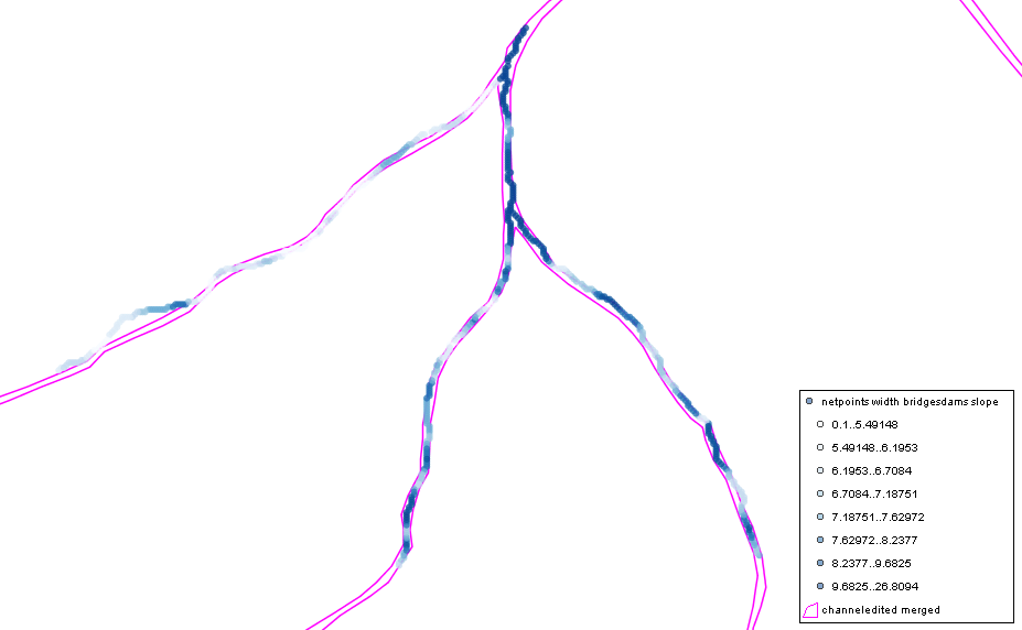
The result of the application of the module for merging and removing holes in the test area is this:

I will start with the development of the next steps: large wood recruitment and propagation downstream.
This week I started the development of the tool for the evaluation of inundation areas using a power law based on bankfull width and channel slope. The parameters of the power law should be derived from field observations and so they have to be input parameters.
The model developed is LW07_NetworkBufferWidthCalculator and it calculates the possible inundated areas considering also the superficial geological formations (only alluvial areas).
The inputs of the model are:
- shapefile of the network points
- shapefile of the bankfull sections
- shapefile of the superficial geological formations: the shapefile should contain the polygons in the areas of interest where there is no rock and erosion phenomena can occur.
The outputs of the model are:
- shapefile of the network points with two additional parameters, average channel slope and possible inundation width
- shapefile of the inundation sections: line segments with the maximum extension of the water calculated using the power law
- shapefile of the inundated areas: polygons of the inundated areas along the channel network -> NOT YET IMPLEMENTED!!
Some notes about the implementation of the model:
- the inundation areas should not be extended where the geological superficial formations is rock because in those parts there isn't the possibility to erode the soil and so there will be no contribution of wood
- the sections that intersect the rock geology in the baricenter of the bankfull will be left as they are, inundated width is the same as bankfull width
- the sections that intersect the rock on the new vertexes should be cut to fill only the areas where there are possible erodible geological formations -> NOT YET IMPLEMENTED!!
- the increased channel width has to be calculated on the original channel section: the bankfull sections have to be extended on both sides to reach the new channel width.
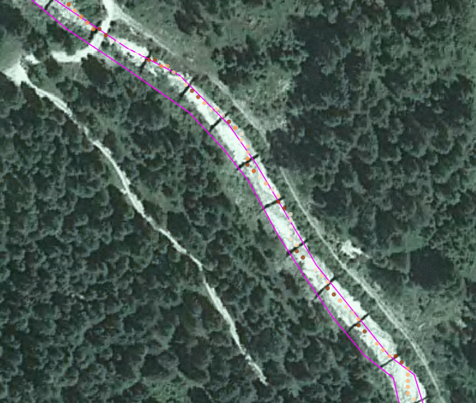
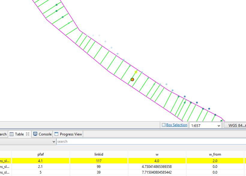
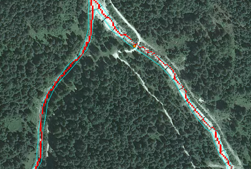
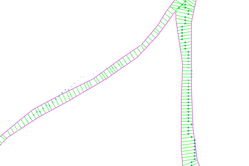
The results of the first implementation of the module on the testarea are the following:
-
the network points with the attribute of inundation width calculated considering the superficial geology

-
the channel sections with the length of inundation width (same as the attribute of the network point) calculated considering the superficial geology
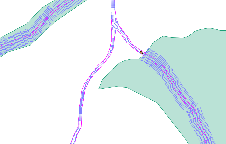
-
the same channel sections visualized on an orthophoto

-
a zoom on a section where there is a fixed value of channel width (bridge or check dam) that can not change due to flooding events (possible critical sections).

I also added some pictures with the results of the analysis to the previous state of the art of the project.
I will go on with the implementation of this module for the missing parts and then finish the design of the development of the next steps: large wood recruitment and propagation downstream.
During this week I:
- continued with the study of the theory for large wood recruitment and propagation downstream
- fixed the bugs in the module for the evaluation of the channel width developed last week
- tested the modules developed until now with a new testcase and found some bugs to fix
- started to develop the module for the evaluation of the average slope in each section.
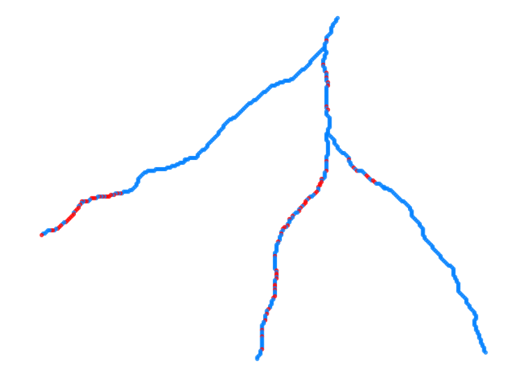
The module developed this week evaluates the local channel slope in each point of the channel network. This is the starting point for the procedure to evaluate the average channel slope in each section considering also the surrounding cells (upstream and downstream).
As you can see the local slope is coherent with what reported in the orthophoto because high values of slope (red dots) are localized where there are dams along the stream network.
The average slope will be calculated in the next module together with the inundation width which requires almost the same background elaborations on channel points.
I had to participate to a conference in Warsaw so I didn't have enough time to go on with the development.
I will go on on the study of the theory for large wood recruitment and propagation downstream and start to develop the module for the evaluation of the average slope and inundation width in each section.
During this week I focused my activities on the definition of the scientific background for LW recruitment and propagation modules. This modules will be developed during the last weeks but before I have to study the theory and define the workflow, since my supervisor at the university will be in vacation during that period.
The new module developed during this week is the module to force the channel width in the sections where there are bridges and check dams. These human structures will modify the natural evolution of channel width and will be (in the propagation phase) the most probable critical sections. Dams and bridges are georeferenced with GPS or other technique and they can be not perfectly on the network extracted from the DTM. The structure is linked to the nearest section on the network within a predefined maximum distance.
The evaluation of the new channel width is done differently for dams and bridges:
- check dams: a fixed, constant width is used
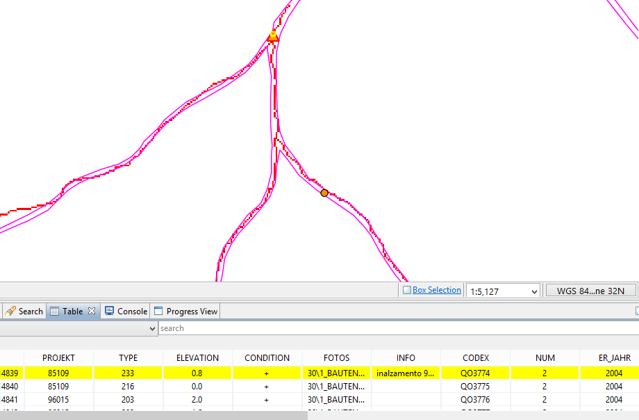
- bridges: the attribute of the bridges layer containing the length is used.

If the bridges do not have the information of their length they will not be considered, but they are added to an output layer with all the problematic bridges. In this way they are easily recognized and in some cases the length of the bridge could be updated by the user before running the simulation again.
The outputs of the module are:
- the network points layer with the attribute of the bankfull width and the width of bridges and check dams

- the layer of bridges without the length attribute.
I will go on on the study of the theory for large wood recruitment and propagation downstream and start to develop the module for the evaluation of the average slope in each section.
There are also some minor fixes to do on the module developed this week.
The module developed during this week is the module to extract the bankfull width for each section of the stream network. Bankfull width is extracted from the bankfull polygon layer.

The inputs of the model are the extracted network and the bankfull polygons and they usually become from different sources:
- bankfull layer is derived from orthofoto, satellite data or hydraulics models
- network layer is usually extracted from DTM using geomorphological functions based on elevation and flow directions.
An example of how different are the two information is the following:
The different origin of the input data can be a source of problems. There are different situations to handle:
- the extracted network is (almost) in the center of the bankfull polygon
- the extracted network is only tangential to the bankfull polygon
- the extracted network does not intersect the bankfull polygon.
I developed specific code to handle all these situations in a way that it is possible to assign the bankfull width to a channel section even if there isn't any intersection between the two. The bankfull width is assigned considering the relative position between the channel point and the bankfull polygon as the width of the bankfull in the nearest point of the channel point. If the channel and the bankfull polygon are too far (maxdist) or if there are others problems to draw the correspondent section, the point is labelled as problematic and added to the output problem point layer.
The outputs of the module are:
- the network points layer with the attribute of the bankfull width
- the sections in the bankfull polygon from which the width is calculated for each point
- the problematic points layer with the points where the program was not able to define a bankfull section.
There is an additional attribute to the main output network point layer which defines the origin of the bankfull width. At present, it is fixed to a value of 0. This value will be updated in the next module to consider if in the section there are human structures that force the bakfull width to a defined width (bridges or check dams).
I will add the possibility to force the bankfull width to a defined width given for human structures along the network (bridges and check dams), the attribute of the network points will be updated to consider the different origin of the channel width.
This week I worked on data preprocessing:
- bankfull layer
- network layer
Bankfull discharge is estimated as a flood with high recurrence frequency (2-years flood or the flood that has a 50% probability of occurring in a given year) Bankfull width represents the river width at the bankfull discharge and usually it is estimated using remote sensing data (orthofoto or satellite images). One of the input of the module to estimate the inundation areas is a layer containing the bankfull polygons for the channels. This input can derive from different sources or also it can be manually drawn. For further analysis it is important that geometries are validated and clean. The first module I developed is used to clean geometries and in particular to merge adjacent bankfull polygons into a single geometry (LW01_ChannelPolygonMerger)
Stream network position is the core of the model, usually it is derived using hydrogeomorphological tools based on DTM, flow direction and total contributing areas and it is a raster layer with information of channel/no channel.
-
JGrassTools library already contains a module which can be used to convert raster network into a vector network with links orientated from upstream (startpoint) to downstream (endpoint) and some attributes, in particular the hierarchical classification of each link of the network. This module is called NetworkAttributesBuilder. The second module I developed is a simple call to the already existing module to create the vector of the network. In this call I set up as constant some fields of the original module that are not used in the following workflow (LW02_NetworkAttributesBuilder)
-
the evaluation of the width of the bankfull and the output inundated areas will be done for each section of the network. Therefore, the third module I developed is a module to extract each point along the network with the original attributes of the line stream and an additional attribute referring to the position of the point in the link (progressive distance of each point from the starting node) (LW03_NetworkHierarchyToPointsSplitter).
I will use the processed input layers (bankfull polygons and channel points) to extract the bankfull width in each section of the stream network.
I dedicated this first week of the Google Summer to:
- set up all the necessary tools to start coding (next week)
- analyse the available modules and the requirements of the new module.
- created (as agreed with my mentor) a fork on GITHUB of the JGrassTools code that will become my working space: https://github.com/silviafranceschi/jgrasstools
- downloaded all the code on my machine as a clone
- downloaded all necessary libraries and created the Eclipse project for all subprojects
- set up the connection between my fork and the original repository by adding a the original repository to the list of my repositories
- identified the package where to add my module: /hortonmachine/hydrogeomorphology
I analyzed the available modules, in particular those related to the extraction of the network attributes, with the requirements of the module I have to develop, and identified the needed additional attributes.